
(click here for introduction and part 1)
A Primer On Mathematical Models In Finance
Let me start by saying what part 2 is not about. It’s not about the spreadsheet models financial analysts use to calculate a target price or fair price for a company’s stock (although I will say a couple of words about them to highlight the contrast). Neither is it about the models (spreadsheet or more sophisticated) that fund managers may use for stock picking or market timing. Both tend to be looked upon by quants as undisciplined and lacking rigor. Most often the mathematics is very basic. Sometimes it’s more involved, but the users are apt merely to use them as a post-hoc rationalization of a decision they’ve already made intuitively.
1. PRICING
The models discussed in this part form the subject of the fast-growing field of mathematical finance, also called quantitative finance. I estimate that more than 90% of the topics covered by quantitative finance involve the pricing of financial derivatives; options, swaps, futures etc. They are called derivatives because their value is derived from the value of other financial securities (e.g. a call option on IBM shares), or from financial variables like interest rates or exchange rates. Knowing the contract terms of such a derivative, how do you determine its value?
Let’s start with a famous quote by Larry Summers parodying financial economics (you can equate financial economics with mathematical finance in the present context):
[Ketchup economists] have shown that two quart bottles of ketchup invariably sell for twice as much as one quart bottles of ketchup (…)[1]
That’s funny, of course. But we should be careful not to mistake caricatures for the real thing. One reason why mathematical finance is a little bit less trivial than the quote suggests is because in finance, it’s not so obvious how much ketchup is in the bottle. And what is in the ketchup to begin with, for many ketchups are a mixture of other, more basic ketchups.
Suppose you want to start a new ketchup company. You must have an idea about what price you’re going to charge customers for your ketchup. That price must be at least your cost price, plus a markup, because you want to make a profit. So you start by estimating how much it’s going to cost your company to produce and sell the ketchup. Your estimate will be guided by the cost price of the ingredients, salaries and the cost of financing your investment in a production plant, to name only a few.
Now suppose that, rather than a ketchup company, you want to start an insurance company, selling life insurance. The biggest component of your costs are the benefits you pay to the beneficiaries when the insured person dies. You know for sure exactly how much you’re going to have to pay (the benefits are fixed in the insurance policy); you just don’t know when. That’s important, because your profit depends on when the insured dies. Not only because of the time value of the benefits (an upfront amount is worth more than a future payment because of the interests you receive when you deposit the upfront amount). More importantly, the time of death matters because the policy holder stops paying the annual premiums once the benefit is paid (upon the insured person’s death).
Clearly, it’s essential that you have an idea about mortality rates before entering the market. By using easily available mortality tables and actuarial science (mathematics of insurance, leaning heavily on probability and statistics), you’re able to work out a fair premium. The fair premium is the premium that balances the premium payments by the policy holder and the benefit payments by the insurance company. On top of the fair premium you add a markup to cover your administrative costs and to pay your shareholders.
The premium being “fair” or ‘balanced” doesn’t mean that each individual beneficiary will receive a benefit (in present-value terms) exactly equal to the sum of the premium payments (also in present-value terms). Then it would not be a life insurance but just a savings deposit. The whole point of an insurance is that not every insurance policy pays back the accumulated premium payments upon the insured person’s death. Some of the insured die young; their beneficiaries receive more. Others die old; their beneficiaries receive less than the sum of premium payments. But it should be true on average, that is, for a large portfolio of insurance policies, early deaths are balanced by die-hard survivors.
It’s easy to understand that being able to calculate a fair premium is crucial for your insurance business. If you charge less than the fair premium, you risk having received too few premiums to pay out the contractual benefits, and you go broke. If you charge too much, you risk selling no insurance policies at all, because your competitors are cheaper.
The basic idea underlying the pricing of financial derivatives is exactly the same as for the manufacturing company or the insurance company: the fair price should cover the costs of selling a product. In finance, the most important part of the cost is the cost of hedging. Let me explain. The purpose of hedging is to take an offsetting position each time[2] a trader buys or sells a derivative, so that the value of the hedge cancels out the value of the initial trade at all times.
For example, if a trader sells a call option to a customer, and hedges her position through the purchase of an identical call option, the price of the sold option should be at least as high as the price of the bought option. That’s as easy as ketchup economics. It’s also easy to understand that that would be a free lunch for the trader. Free lunches in this perfect, obvious form may not be literally non-existent, but they are sufficiently rare that ‘hunting for free lunches’ is rarely a viable business model[3]. The example also begs the question as to what a fair price for the option is.
But there’s another, more roundabout way to hedge; namely through a sale or purchase of the derivative’s underlying asset. The easiest way to explain this is by taking a forward contract as example. Suppose a Russian customer of a European bank wants to buy 1 million euros against rubles, not today, but one year from now. By buying the euro “forward”, the customer can fix the euro/ruble exchange rate today, so that he doesn’t have to worry about how many rubles he’ll have to pay for the euro amount. Suppose today’s (“spot”) rate is 40 rubles for 1 euro (40/1).
You might expect the one-year forward rate to be the same as today’s spot rate, but not too fast. If one year hence, the euro/ruble rate is 1 to 45, the bank would be required to deliver EUR 1 million, but would receive only RUB 40 million from the customer, rather than the market rate of 45 million. That’s a loss of RUB 5 million. How to avoid that loss?
The bank could ask some economist to predict what the exchange rate will be one year from now (based on economic, political and/or other analyses). But trust me, such predictions are notoriously unreliable. There is, however, a much easier way to determine a fair forward price; one that precludes the necessity to make predictions – one that uses only currently and easily available information in a very direct way. Let’s see how.
The uncertainty the bank faces is in how many euros it can get when it sells the rubles (which it receives from the customer) in the market. Rather than waiting one year to sell them, it could sell them already now, in order to remove any uncertainty about future exchange rates. Unfortunately, the bank doesn’t have rubles to sell now. No problem, it just borrows rubles in the market, sells them immediately, and deposits the euro proceeds on a fixed rate euro account. The bank’s transactions are schematized in the following diagram:
Bank’s transactions on day 1:
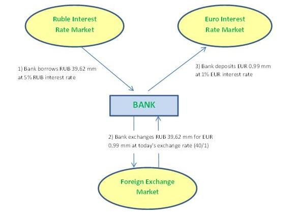
The bank has to repay its RUB debt at the end of the year, plus interests. That’s an extra cost which it has to take into account. On the other hand, it will receive 1% on its EUR deposit, so that’s an extra gain it can subtract from its costs. If the bank subsequently puts the forward rate at RUB 41.6 million, the following diagram shows that the rub/eur forward trade combined with the spot transactions on day 1 (the hedge) leads to a break-even at the end of the year, whatever the exchange rate is at that moment:
Bank’s transactions after one year:
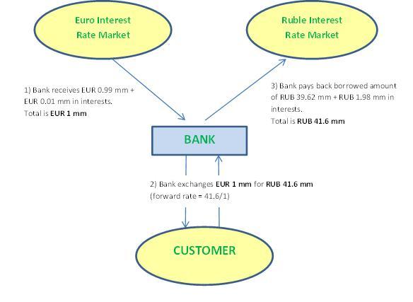
The 41.6/1 forward rate can be calculated directly from the spot rate (40/1) and the RUB and EUR interest rates (5% and 1% respectively) as follows:
Forward rate = Spot rate × (1 + RUB rate) / (1+ EUR rate)
= 40 × (1 + 0.05) / (1 + 0.01) ≈ 41.6
Every cash-flow in this diagram is fixed in advance; there is no uncertainty about any amount the bank will pay or receive. This is the crucial thing to understand: when determining the forward rate, the bank doesn’t need any expectations[4] about how the exchange rate will move. The bank just works out how it should set up the hedge, and sets the forward rate so that all its present and future cash-flows are matched by cash-flows in the opposite direction. That’s the essence of quantitative finance: by finding a suitable hedge you determine the derivatives price such that the cash-flows from the derivative are always matched by the cash-flows from the hedge, for all possible future market scenarios. Stated otherwise, quantitative finance attempts to relate the price of one asset (e.g. foreign exchange forward) to the price of (an)other asset(s) (e.g. RUB and EUR deposits). So that’s what Larry Summers had in mind.
That fundamental principle is similar to the pricing of bets by bookmakers. The bookmaker will try to balance his book, i.e. to price his bets in such a way that, whatever the outcome of the game is, he will not lose money. He’ll have to pay the winning bettors of course. But that’s OK, as long as he can keep enough money off the losing bettors. By hedging his bets, he doesn’t care who wins the game. Neither does the trader care whether stock prices go up or down, as long as his positions are properly hedged.
But there is a rub (no pun intended). In the RUB/EUR forward example, the solution is almost trivial, and the hedge can be considered perfect[5]. But for more complicated derivatives, especially options, you need to make some additional assumptions, and a hedge using non-identical assets always carries some residual risk.
Although you still don’t need to know what the exact price of stock ABC or exchange rate XYZ will be one year hence, you do need some assumptions about the range of possible values (based on the stock price or exchange rate volatility, for example). For that, you need more than ketchup economics. You need mathematical models.
Not any model will do, of course; some models are better than others. The direct implication is that the price of an option (for example) is model-dependent. That is, different models yield different prices. I will not here go into the subject of which models are good, and which aren’t. But in part 3 I will argue that the importance of model assumptions is often exaggerated. The main take-away for the moment is that derivatives pricing does not involve making predictions as to whether prices will go up or down. If your positions are properly hedged, you don’t care where the market is going. The value of your positions will be the same in every conceivable scenario.
So yes, markets are unpredictable, even to a high degree (though not completely, as we will see in a moment). But that has little bearing on a quant’s work, in terms of limiting her capacity to price financial securities (see indented text below: Error revisited).
Error Revisited
Financial models are typically stochastic, which means that randomness is an inherent part of the model. Similar to the error term we’ve seen in the height-weight example in part 1, financial equations also contain an explicit random component. Let’s look at arguably the most famous stochastic equation in finance: Geometric Brownian Motion (underpinning the Black-Scholes formula for option pricing).
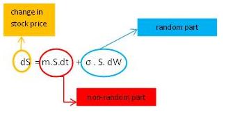
The formula attributes the change in the stock price (dS) to a non-random part (the first term, which can be interpreted as being determined by the long-run average return), and a random part (the second term). Basically this means that in the long run, stock prices can be expected to move in a certain (usually upward) direction. But there is a great deal of uncertainty as to what exactly a particular stock will be worth in one month, in one year, or in ten years. That uncertainty is captured by the second term (the error term in the terminology of part 1).
Let’s make the comparison with the height-weight example more explicit:
Weight = 74 kg + e (model 1)
We know that the average weight of an American adult is 74 kg. That’s the non-random part. But most Americans have a different weight. That’s why we have to add a random component, the ‘e’. That sounds like a convoluted way to specify someone’s weight (“Tom’s weight is 68 kilos; namely 74 kg – 6 kg”). But the point of the model is not to describe a particular individual’s weight. The point is to reveal patterns in the distribution of weights among the population.
Similarly, the stochastic equation is not used to explain individual stock price movements. But even if it can’t be used to make exact predictions about the future price of each stock traded in the market, it is still useful to reveal general patterns in market fluctuations.
The brilliant insight of Black, Scholes and Merton, the eponymous inventors of the famous option pricing formula, was that by adding the underlying security to the equation, you can make the random term disappear, so that the option price can be calculated from the price of the underlying stock (and some additional, non-random, parameters). As a result, the option price contains no more randomness than is already present in the stock price.
Before moving to the next section, I would like to add a few comments about trading. In the popular media trading is often equated with gambling. And for that reason it should be banned – in the opinion of (mostly uninformed) commentators. Granted, activities of traders have led to some spectacular losses in the past, on some occasions with dramatic consequences for depositors. But not all trading is equal. And the requirement that banks stop taking risks altogether is not only misguided, but also impossible, for risk is an inherent part of any business. What exactly are the risks involved in trading?
An important distinction to be made is between proprietary trading (“prop trading“) and market-making. Prop traders take active bets, for example that volatility is going to rise, or interest rates going to fall. They can be said to speculate, unlike their colleagues in the market-making trading desks. A market maker doesn’t bet at all. As explained above, the market maker plays an intermediary role, matching buyers with sellers, just like a second-hand car dealer does. Of course that’s not without risk, because exactly like the second-hand car dealer the market maker always runs the risk of not finding a buyer willing to pay at least the same price. But if we should call something gambling just because it involves risk, then all forms of investing and economic activity in general should be called gambling. That would make the word totally uninformative. Keep in mind that many derivatives serve useful economic purposes, like a farmer wishing to hedge himself against falling prices for his produce (e.g. by selling futures).
Using blanket terms like gambling indiscriminately is not very helpful either if we want to figure out what trading activities should be restrained, and in what way. For example, I think it makes sense to create a wall between an institution’s prop trading and its regular banking activities (e.g. savings deposits). That can be done by prohibiting prop trading desks from speculating with money the bank collected from its depositors.
As for the economically more beneficial market-making form of trading, some regulation might be advisable here too. Like requiring banks to make sure their positions are sufficiently hedged, and any remaining risks properly contained and monitored. Or banning the sale of highly complex financial products to non-professional customers (who usually end up paying too much for something they don’t understand and often contains significant hidden risks). There are several reasonable measures that can be taken to thwart excessive risk-seeking behavior. Taking potshots at a broad category of people engaged in ‘risky’ activities is not one of them. Only informed decisions have the potential to make things better and safer.
2. RISK MANAGEMENT
The essential lesson from the previous section is that quants, when pricing derivatives, don’t need to have any idea about where asset prices are going – up or down. For the purposes of risk management, however, a quant does make some predictions. But those predictions are much weaker than many accounts in the popular media suggest. The risk manager is not asked to predict what the price of stock ABC will be in the future. She’s not even asked to give her opinion about whether equity prices will move up or down. Usually, one of her tasks involving some sort of prediction is to provide a worst-case scenario. Let’s look at an example.
The left half in the figure below plots the 12-month price history of an equity index. It was at 100 points 12 months ago. And today (where the red curve crosses the blue one) it’s at 112. From that point the blue curve turns into a straight line[6]. The right half shows the forecasted prices for the next 12 months. The blue curve in that part is the ‘expected’ price evolution for the next 12 months. Expected is a technical term in statistics (not to be confused with its vernacular meaning); roughly meaning the center point in a range of possibilities, like an average. It doesn’t mean that statisticians literally expect the price to go from 112 to 114.25 points in an (almost) straight line over the next 12 months. Here it can be loosely interpreted as: from all the possible paths the index can take, this is more or less the center path.
One-year historical price path of an equity index and forecasts for the following year:
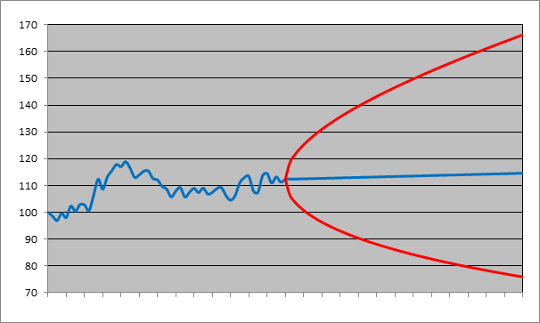
The red curve delimits a prediction (or confidence) region. The true but yet unknown path the index will take in the next 12 months will be an erratic curve as in the previous 12 months, but it is predicted to remain within the area delineated by the red curve. Even that is not strictly true: the prediction is made with a certainty of 95%. If you want a higher certainty, the prediction region, in other words the range of possible values, widens. If you want 100% certainty, the index will be between 0 (total loss) and plus infinity (the index doesn’t have an upper bound).
The forecasts are based on a lognormal model (drift = 2%; volatility = 20%). Yes, the model so much vilified by Taleb and his acolytes. If you use another model, or other values for the drift and volatility, you get different results. Regardless of whether the lognormal model is appropriate or not, the point I want to make here is that any realistic model will show a similar picture: lots of uncertainty about future prices, and the uncertainty increases with time[7]. Also, what’s important is the red curve, not the blue one. You will never hear a statistician ‘predict’ that the index will be 2% higher one year from now. Rather, she will predict that the index will be between 75.9 and 166.2 points, with 95% certainty.
Incidentally, note the important difference with the target prices with which stock analysts entertain an eager audience. As said in the introduction, stock analysts may use some sort of spreadsheet model yielding a target price, but most often it’s just a price that is in the neighborhood of the current price (some tweaking of the input variables in the spreadsheet may be needed to make sure the target price is not too far off from the current price or the target prices from other analysts). Research confirms that target prices are a lagging rather than leading indicator of future stock prices. In other words, target prices are revised upwards not because the company’s future looks brighter, but merely because its stock price has already significantly increased.
The statistician’s predictions may be much more tentative, but on the other hand she’s not allowed that non-committal attitude generally adopted by stock analysts towards their target prices. What I mean is this: a stock analyst can always find some excuse if the stock price doesn’t reach his target price (“Of course I didn’t mean to say that the price would increase to exactly $ 25 !!”). But the statistician’s predictions can be tested: if she predicts that future prices will remain within the 95% confidence region, then in 95% of cases, they should. So if the price falls outside the region in much more than 5% (= 100% – 95%) of observed cases, it means there’s a problem with her model. This also shows that a probability of 95% in statistics has a both precise and testable meaning, unlike informal statements like “I’m 95% sure I forgot to add salt”.
To sum up, statisticians don’t predict prices, they predict possible ranges of prices, with a stated probability that the price will remain within that range. If you’re an investor and you look to a model to tell you if the market is going up or down, you’re likely to be disappointed. The model doesn’t tell you that. What’s the point of a model then, if you can’t use it as an investor?
Well, my first answer is that predicting the behavior of maybeetles in the mating season is not of much use to investors either; still some scientists devote their attention to it. You see, the whole world doesn’t revolve around the investor (although some degenerate specimens of homo investus might think it does). An academic researcher’s main concern lies not with the question whether her work is directly useful to some particular group of people, but whether it contributes to a better understanding of the world and its inhabitants. That holds for finance as much as for biology.
Then again, shouldn’t the work done by quants working in financial institutions be useful, to those institutions? Yes, of course. So here’s my second answer: the investor does get useful information from the model. If not the exact future return he can expect, at least he gets an idea about what’s possible, to the upside as well as to the downside. A model thus tells you something about the risk of an investment. For a conservative investor, for example, the 32% possible loss in one year’s time could be too much to consider investing in the index.
So the lesson of this second section is that admitting asset prices are unpredictable does NOT imply all predictions are totally unreliable, or that trying to model asset prices is futile. Even in the face of uncertainty, it’s possible to find some structure, some pattern in what may look as complete randomness. Just specifying the magnitude of the uncertainty (e.g. by indicators such as volatility) is already far more informative than saying prices can go anywhere.
Summary of part 2 (and preview to part 3): Quantitative financial models are not used to predict stock prices. Their main uses are in pricing financial derivatives and in risk management. In both areas, the answers given by quants are model-dependent to some degree. Thus, choosing an appropriate model and correctly specifying its parameters is important, but it’s equally important to keep in mind what the model is used for. A model may be more “correct” in some abstract philosophical sense, but it may be so impractical as to render it useless. That will be the subject of part 3.
[1] Lawrence H. Summers, The Journal of Finance, Vol. 40, No. 3, Papers and Proceedings of the Forty-Third Annual Meeting American Finance Association, Dallas, Texas, December 28-30, 1984 (Jul., 1985), pp. 633-635
[2] Not literally each time. Hedging is usually done globally; for an entire trade book, rather than for each separate trade.
[3] The activity of market makers may seem to come close. What prevents market-making from being a truly free lunch, however, is the fact that they must provide liquidity (they need to fund their activities), and they always run the risk of not finding a buyer or seller to take the other side of their trade at the same price they entered into it. In addition, they run the risk that the counterparty they bought the call option from goes bankrupt, so that they lose the positive side (bought option) of the hedged trade, but remain stuck with the negative side (option sold to the initial customer).
[4] In the media you can hear statements like: “Judging from the RUB/EUR futures (a future is similar to a forward contract), the market expects the euro to increase relative to the ruble.” I avoid such statements because they are misleading. The forward (or futures) rate merely reflects current market conditions, like spot rates and rates for borrowing and lending. The word ‘expect’ comes from an overly literal interpretation of the artificial, so-called risk-neutral probabilities used in pricing derivatives. Quantitative finance is allowed to use such “unreal” probabilities because they lead to exactly the same price as hypothetical real-world probabilities would. But the word ‘expectation’ in that sense has a very narrow technical meaning, and it has nothing to do with what the participants in the market really expect.
[5] The bank is only perfectly hedged under the assumption that the customer doesn’t default. In a default scenario, the bank can still incur losses if it has to close the hedge position at unfavorable rates.
[6] Strictly speaking, the line is slightly curved, but the curvature is barely noticeable.
[7] In mean-reverting models, though, the red curve may converge to an upper bound different from infinity and to a lower bound different from zero.